Rendering a scanning 3DXRD dataset

The renderer turns a grain map into the detector frames that a scanning 3DXRD experiment would record. It renders one dty row at a time, and anri.io.simulate_sparse runs it for every row of a scan, writing ImageD11’s sparse pixel format. ImageD11 can then process the simulated data like real data.

This notebook goes through what the renderer does, one step at a time, on a small phantom:

1. Select which peaks can reach the row. A peak is one (map entry, hkl, Friedel branch) combination.

2. Model each peak as a 3D Gaussian in (slow, fast, \(\omega\)): the centroid comes from the forward model, and the covariance from propagating the spreads of the beam through it.

3. Integrate each Gaussian over a small window of detector cells (frames × pixels).

4. Weight each peak by its intensity factors: density, \(|F|^2\), Lorentz, polarisation, and how much of the voxel the beam illuminates in each frame.

5. Merge all peaks into one list of sparse pixels.

import anri.utils
anri.utils.setup()  # before any JAX computation: don't grab most of the GPU memory at start-up

import os
import tempfile
import time

import jax
import jax.numpy as jnp
import numpy as np
from matplotlib import pyplot as plt
from ImageD11.sinograms.tensor_map import TensorMap

import Dans_Diffraction

import anri.crystal, anri.fwd, anri.io

start = time.time()

The map

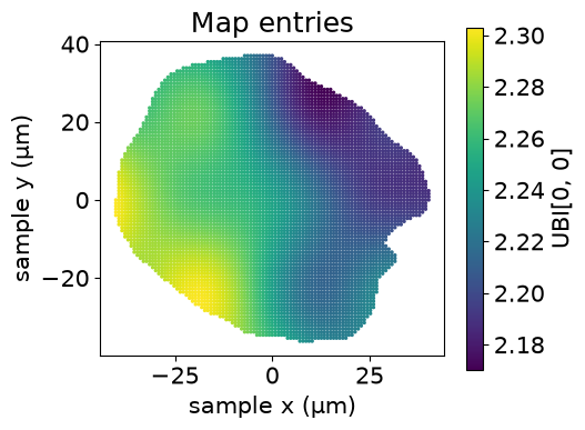
The renderer takes a map as a flat list of entries, each with a position in the sample frame, a UBI matrix and a density. Nothing requires one entry per voxel: a voxel can have several entries, e.g. for two orientations. The renderer handles one phase at a time, so a multi-phase map is rendered phase by phase.

Our phantom is one slice of a deformed \(\alpha\)-quartz grain, with intragranular misorientation and strain, from flyxdm (see tests/data/phantoms/quartz_flyxdm/README.md). It is stored as an ImageD11 TensorMap, and anri.io.entries_from_tensormap turns it into entries:

tmap = TensorMap.from_h5("../../../tests/data/phantoms/quartz_flyxdm/quartz_flyxdm_tmap.h5")
entries = anri.io.entries_from_tensormap(tmap)
print({k: v.shape for k, v in entries.items()})

fig, ax = plt.subplots(figsize=(5, 5))
sc = ax.scatter(entries["pos"][:, 0], entries["pos"][:, 1], s=2, c=entries["ubi"][:, 0, 0])
fig.colorbar(sc, ax=ax, shrink=0.8, label="UBI[0, 0]")
ax.set(aspect=1, xlabel="sample x (µm)", ylabel="sample y (µm)", title="Map entries")
plt.show()

{'ubi': (6818, 3, 3), 'pos': (6818, 3), 'density': (6818,)}

Crystallography

Each peak needs its hkl and its structure factor \(|F|^2\). anri.crystal.reflections lists every hkl separately (not merged into rings), and anri.crystal.structure_factors gives \(|F|^2\) for each.

wavelength = 0.2845704100778472  # angstrom, as in the flyxdm simulation
xtl = Dans_Diffraction.Crystal("../../../tests/data/cif/SiO2.cif")
refl = anri.crystal.reflections(anri.crystal.lattice_parameters(xtl), anri.crystal.space_group(xtl), wavelength, 1.0)
F2 = anri.crystal.structure_factors(xtl, refl["hkl"], wavelength)
strong = F2 > 0.01  # drop the reflections the atom positions extinguish
hkls = refl["hkl"][strong].astype(float)
F2 = F2[strong]
print(len(hkls), "hkls")

446 hkls

/tmp/ipykernel_6019/348910026.py:4: UserWarning: No isotropic thermal factors (U_iso or B_iso) for SiO2: intensities have no Debye-Waller attenuation.
  F2 = anri.crystal.structure_factors(xtl, refl["hkl"], wavelength)

Geometry

anri.io.geom_from_pars builds the geometry from ImageD11 parameters (detector, beam and goniometer). Note that ImageD11’s wedge has the opposite sign to anri’s. On top of those, the renderer needs the things that set the peak shapes and weights:

parameter	meaning
sig_wavelength	standard deviation of the wavelength (Å)
sig_ky, sig_kz	standard deviations of the horizontal and vertical beam divergence (radians)
sig_beam, width_beam	the beam’s profile across it, horizontally: a flat top of width_beam (default 0, a Gaussian) blurred by a Gaussian of sig_beam (same units as dty, here µm)
sig_beam_v, width_beam_v	the same vertically; only needed for 3D maps of cube voxels (voxel_3d=True), as a 2D map’s voxels are columns that the whole vertical profile crosses
voxel_size	side length of the (square) voxels, same units as dty
pol_factor	degree of horizontal polarisation, 1 for a fully horizontally polarised beam
sig_psf	standard deviation of the detector point spread (pixels)

pars = {
    "y_center": 1049.9, "y_size": 75.0, "tilt_y": 0.0,
    "z_center": 1116.5, "z_size": 75.0, "tilt_z": 0.0, "tilt_x": 0.0,
    "distance": 150e3, "o11": -1, "o12": 0, "o21": 0, "o22": -1,
    "wavelength": wavelength, "wedge": 0.0, "chi": 0.0,
}
det_shape = (2162, 2068)  # (slow, fast) pixels

geom = anri.io.geom_from_pars(
    pars, y0=0.0, sig_wavelength=wavelength * 1e-4, sig_ky=1e-4, sig_kz=1e-4,
    sig_beam=0.5, voxel_size=float(tmap.steps[1]), sig_psf=0.3,
)

The row

A dty row is one ImageD11 scan: a series of frames, each with its own \(\omega\) and dty. anri.fwd.make_row sorts the frames by \(\omega\) and puts each frame’s edges halfway between neighbouring \(\omega\) values, so frames don’t have to be evenly spaced or recorded in order. Here we take one row at dty = 0: 180° of rotation in 0.25° steps.

ostep = 0.25
omega = np.arange(0.0, 180.0, ostep) + ostep / 2  # frame centres
row = anri.fwd.make_row(omega, dty=np.zeros_like(omega))
print(len(omega), "frames, omega from", row["omega_min"], "to", row["omega_max"])

720 frames, omega from 0.0 to 180.0

Step 1: which peaks reach this row?

Every (entry, hkl, branch) is a candidate peak. The branch picks one of the two \(\omega\) solutions of the Ewald condition (etasign = +1 or -1, ImageD11’s omega1 and omega2).

For each candidate, anri.fwd.select_peaks computes the centroid (slow, fast, \(\omega\)) with the voxel at its real position for the row’s dty, and keeps the peak if its centroid is within a margin of the row (on the detector, inside the \(\omega\) range) and its voxel is within reach of the beam at that \(\omega\): no further from the beam’s centre line than half its width + \(4\sigma\) + one voxel. anri.fwd.render_row does this for you. We call it directly here to look at the result:

window = (3, 7, 7)  # (frames, slow, fast) cells per peak: render_row's default
margin = jnp.array([
    window[1] // 2 + 1,                         # slow (pixels)
    window[2] // 2 + 1,                         # fast (pixels)
    (window[0] // 2 + 1) * ostep,               # omega (degrees)
    geom["width_beam"] / 2 + 4 * geom["sig_beam"] + geom["voxel_size"],  # distance from the beam, across it
    geom["width_beam_v"] / 2 + 4 * geom["sig_beam_v"] + geom["voxel_size"],  # and vertically (cubes only)
])
ent = {k: jnp.asarray(v) for k, v in entries.items()}
geom_j = jax.tree.map(jnp.asarray, geom)
row_j = jax.tree.map(jnp.asarray, row)

mask = anri.fwd.select_peaks(ent["ubi"], ent["pos"], jnp.asarray(hkls), geom_j, row_j, margin, det_shape)
e, h, b = np.nonzero(np.asarray(mask))  # entry, hkl and branch of each selected peak
print(f"{mask.size} candidate peaks, {e.size} reach this row")

6081656 candidate peaks, 309685 reach this row

Most candidates never reach this row: at the \(\omega\) where they diffract, the beam is passing through a different part of the sample.

Step 2: one peak as a Gaussian

A peak’s centroid comes from the forward model, as in the simple forward model tutorial. Its covariance comes from propagating sig_wavelength, sig_ky and sig_kz through the same model with a Jacobian, as in the forward model covariance tutorial. The spread of the origin over the voxel is not propagated. The voxel’s extent and the beam profile enter through the dty weight instead (step 4). The detector point spread is then added to the slow and fast variances, plus a tiny floor so that a peak with no broadening at all still renders.

The renderer puts each voxel at its real position for the row’s dty. Our row is at dty = \(y_0\) = 0, where that is just the voxel’s sample position rotated by \(\omega\), so the box-beam forward model, anri.fwd.get_centroid_box, gives the renderer’s centroid, and anri.fwd.propagate_cov_box its covariance.

Let’s take a peak from the voxel nearest the centre of the map that is fairly broad in \(\omega\):

g = geom_j
beam_and_gonio = (g["wavelength"], g["k_in_lab"], 0.0, 0.0, g["wedge"], g["chi"])  # ky = kz = 0: no divergence offset
detector = (g["s_step_lab"], g["f_step_lab"], g["det_origin_lab"])
cov_in = anri.fwd.get_cov_in(jnp.zeros(3), g["sig_wavelength"], g["sig_ky"], g["sig_kz"])  # origin spread 0, see above

def peak_centroid_and_cov(i):
    ubi, pos, hkl, etasign = ent["ubi"][e[i]], ent["pos"][e[i]], jnp.asarray(hkls[h[i]]), 1.0 - 2.0 * b[i]
    centroid, valid = anri.fwd.get_centroid_box(ubi, pos, hkl, etasign, *beam_and_gonio, *detector)
    cov = anri.fwd.propagate_cov_box(ubi, pos, hkl, etasign, *beam_and_gonio, *detector, cov_in)
    return np.asarray(centroid), np.asarray(cov)  # (slow, fast, omega) and its 3 x 3 covariance

centre = np.argmin(np.linalg.norm(entries["pos"], axis=1))
best, best_sd = None, 0.0
for i in np.flatnonzero(e == centre):
    c, cov = peak_centroid_and_cov(i)
    sd_omega = np.sqrt(cov[2, 2])
    inside = 100 < c[0] < det_shape[0] - 100 and 100 < c[1] < det_shape[1] - 100 and 5 < c[2] < 175
    if inside and best_sd < sd_omega < 0.2:
        best, best_sd = i, sd_omega
i = best
centroid, cov = peak_centroid_and_cov(i)

# (slow, fast, omega) covariance, plus the point spread on slow and fast.
# The renderer's floor (1e-4 px², 1e-8 deg²) is far smaller than these variances, so we leave it out here.
cov3 = cov[:3, :3] + np.diag([geom["sig_psf"] ** 2, geom["sig_psf"] ** 2, 0.0])
ss, ff, oo = np.diag(cov3)
sf, so, fo = cov3[0, 1], cov3[0, 2], cov3[1, 2]

print("hkl", hkls[h[i]], "etasign", 1 - 2 * b[i])
print("centroid (slow, fast, omega):", centroid.round(3))
print("standard deviations (px, px, deg):", np.sqrt(np.diag(cov3)).round(3))
print("correlations slow-fast, slow-omega, fast-omega:",
      (np.array([sf, so, fo]) / np.sqrt([ss * ff, ss * oo, ff * oo])).round(2))

hkl [-2. -1.  0.] etasign 1
centroid (slow, fast, omega): [ 759.797 1061.318  137.634]
standard deviations (px, px, deg): [0.368 0.374 0.18 ]
correlations slow-fast, slow-omega, fast-omega: [0.15 0.58 0.25]

Step 3: integrating over a window

Each peak gets a fixed-size window of cells (frames, slow pixels, fast pixels), centred on the cell that holds its centroid. The default is (3, 7, 7). Because every peak has the same window size, batches of peaks have fixed array shapes, so they can be compiled once, vectorised and split over devices.

Integrating a correlated 3D Gaussian over boxes has no closed form, so the renderer factorises it by conditioning:

1. :math:`omega`: the mass of the Gaussian in each frame, and the mean and variance of \(\omega\) within that frame (a truncated normal).

2. slow given :math:`omega`: a 1D Gaussian, whose mean shifts with that within-frame mean of \(\omega\).

3. fast given slow and :math:`omega`: likewise, using the within-pixel mean of slow.

Conditioning on the within-cell means, rather than the cell centres, keeps peaks that are narrower than a frame or a pixel at the right position. It also keeps the correlations between slow, fast and \(\omega\): the wavelength spread, for example, smears a spot radially along its Debye-Scherrer ring.

Let’s render our peak with the default window and with two more frames. The captured output is the fraction of the Gaussian that falls inside the window:

one = (e[i : i + 1], h[i : i + 1], b[i : i + 1], ent, jnp.asarray(hkls), jnp.asarray(F2), geom_j, row_j)
for w in [(3, 7, 7), (5, 7, 7)]:
    frame, pixel, value, captured = anri.fwd.render_peaks(*one, w, det_shape)
    print(f"window {w}: captured {float(captured[0]):.4f}")

window (3, 7, 7): captured 0.9628
window (5, 7, 7): captured 0.9995

This peak is broad in \(\omega\), so three frames lose a few percent of it. anri.fwd.render_row returns captured for every peak, so you can check this and enlarge the window if needed.

To check this, we simulate the peak directly: draw the wavelength and beam divergence from their spreads, push every sample through the forward model, add the point spread, and histogram the (slow, fast, \(\omega\)) positions into the same cells. This tests the linearised covariance as well as the integration over the window. Within a row, the per-peak and per-frame factors (step 4) are the same in every cell of a window, so the rendered values divided by their total, times captured, are the rendered fraction of the peak in each cell:

w = (5, 7, 7)
frame, pixel, value, captured = anri.fwd.render_peaks(*one, w, det_shape)
value = np.asarray(value).reshape(w)
pixel = np.asarray(pixel).reshape(w)
frames_in_file = np.asarray(frame).reshape(w)[:, 0, 0]
rendered = value / value.sum() * float(captured[0])  # fraction of the peak in each cell

# the window's cells: pixel (0, 0) of the window, and the frame edges in sorted-omega order
s0, f0 = divmod(int(pixel[0, 0, 0]), det_shape[1])
jo = np.searchsorted(row["omega_edges"], centroid[2]) - 1 - w[0] // 2
edges = [s0 - 0.5 + np.arange(w[1] + 1), f0 - 0.5 + np.arange(w[2] + 1), np.asarray(row["omega_edges"])[jo : jo + w[0] + 1]]

# Monte Carlo: beam spreads through the forward model, then the point spread
n = 1_000_000
rng = np.random.default_rng(0)
spreads = rng.standard_normal((n, 3)) * [geom["sig_wavelength"], geom["sig_ky"], geom["sig_kz"]]
ubi, pos, hkl, etasign = ent["ubi"][e[i]], ent["pos"][e[i]], jnp.asarray(hkls[h[i]]), 1.0 - 2.0 * b[i]

def sample(wavelength, ky, kz):
    return anri.fwd.get_centroid_box(ubi, pos, hkl, etasign, wavelength, g["k_in_lab"], ky, kz, *beam_and_gonio[4:], *detector)[0]

samples = np.array(jax.jit(jax.vmap(sample))(geom["wavelength"] + spreads[:, 0], spreads[:, 1], spreads[:, 2]))
samples[:, :2] += geom["sig_psf"] * rng.standard_normal((n, 2))
mc = np.moveaxis(np.histogramdd(samples, bins=edges)[0], 2, 0) / n  # (frame, slow, fast) like the window

vmax = max(rendered.max(), mc.max())
fig, axs = plt.subplots(2, w[0], figsize=(2.2 * w[0], 4.8), constrained_layout=True)
for k in range(w[0]):
    for ax, img, name in ((axs[0, k], rendered[k], "rendered"), (axs[1, k], mc[k], "Monte Carlo")):
        ax.imshow(img, vmin=0, vmax=vmax)
        ax.set(title=f"frame {frames_in_file[k]}\n{name}" if name == "rendered" else name, xticks=[], yticks=[])
plt.show()

print(f"largest difference in any cell: {np.abs(rendered - mc).max():.4f} of the peak (Monte Carlo noise ~{np.sqrt(mc.max() / n):.4f})")
print(f"inside the window: rendered {float(captured[0]):.4f}, Monte Carlo {mc.sum():.4f}")

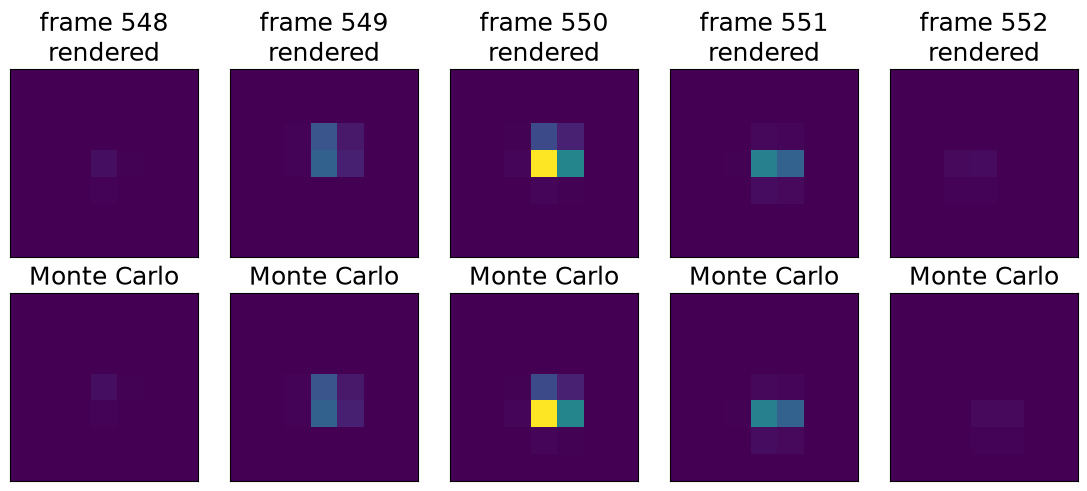
largest difference in any cell: 0.2785 of the peak (Monte Carlo noise ~0.0005)
inside the window: rendered 0.9995, Monte Carlo 0.9995

They agree to within the Monte Carlo noise.

anri.fwd.check_render runs this check for a random sample of peaks from your own map and geometry, and reports, for each, the largest difference in any cell and the fraction inside the window both ways:

check = anri.fwd.check_render(entries, hkls, geom, row, det_shape, window=window, n_peaks=100, n_samples=100_000)
err = check["max_cell_error"]
print(f"{len(err)} peaks: largest cell difference, median {np.median(err):.4f}, 99th percentile {np.percentile(err, 99):.4f}, max {err.max():.4f} of the peak")
print(f"largest difference in the fraction inside the window: {np.abs(check['captured'] - check['captured_mc']).max():.4f}")

99 peaks: largest cell difference, median 0.0018, 99th percentile 0.2569, max 0.5122 of the peak
largest difference in the fraction inside the window: 0.0009

With 100 000 samples per peak, the Monte Carlo noise in a bright cell is about 0.002 of the peak, so these differences are mostly noise.

Step 4: intensity

The value of a peak in a cell is

\[\text{density} \times |F|^2 \times L \times P \times w_\text{beam}(\text{frame}) \times T(\text{frame}) \times \text{(fraction of the Gaussian in the cell)}\]

• \(L\) is the Lorentz factor for rotation about the \(\omega\) axis, \(1 / |\hat{\omega} \cdot (\hat{k}_\text{in} \times \hat{k}_\text{out})|\). For a vertical axis this is \(1 / (\sin 2\theta\, |\sin\eta|)\), the inverse of ImageD11’s lf.

• \(P\) is the polarisation factor, which matches ImageD11’s polarization.

• \(T\) is an optional transmission per frame, passed to make_row.

• \(w_\text{beam}\), from anri.fwd.beam_weight, is how much of the voxel the beam illuminates in that frame (its dty moves the voxel across the beam). For a square voxel of side \(a\), rotated by \(\omega\), the length of beam path through it is a trapezoid as a function of the distance across the beam, of area \(a^2\). The renderer convolves it with the beam’s profile across it, a flat top blurred by a Gaussian, in closed form. The profile integrates to 1, so a wider beam spreads the same flux. For cubes (3D maps), the vertical profile is integrated over the cube’s height too.

distance = np.linspace(-2.5, 2.5, 501)
voxel_at = jnp.stack([jnp.zeros_like(distance), distance, jnp.zeros_like(distance)], axis=1)  # across the beam (lab y)
weight = jax.vmap(anri.fwd.beam_weight, in_axes=(0, None, None))
beams = [
    ("narrow beam, $\\sigma$ = 0.05 µm", 0.05, 0.0),
    (f"this notebook's beam, $\\sigma$ = {geom['sig_beam']} µm", geom["sig_beam"], 0.0),
    ("flat top 3 µm wide, $\\sigma$ = 0.05 µm", 0.05, 3.0),
]
fig, axs = plt.subplots(1, 3, figsize=(14, 3.5), constrained_layout=True)
for ax, (title, sig, width) in zip(axs, beams):
    beam = dict(geom_j, sig_beam=sig, width_beam=width)
    for om in (0.0, 30.0, 45.0):
        ax.plot(distance, weight(voxel_at, om, beam), label=f"$\\omega$ = {om:.0f}°")
    ax.set(title=title, xlabel="voxel's distance from the beam's centre (µm)")
axs[0].set(ylabel="$w_\\mathrm{beam}$")
axs[0].legend()
plt.show()

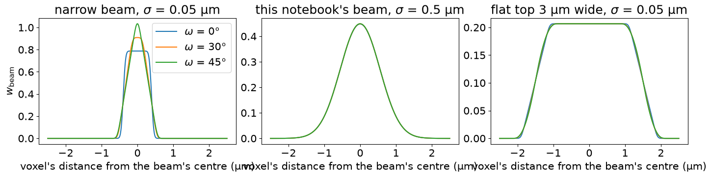
With a narrow beam, you can see the voxel’s trapezoid (a rectangle at \(\omega\) = 0°, a triangle at 45°). A beam wider than the voxel smooths that out, and a flat-top beam wider than the voxel lights it fully over most of its width. Integrated over the distance, the weight is always the voxel’s area.

Pencil, line and box beams are all set this way: narrow or wide, Gaussian or flat-top, in each direction.

Step 5: a whole row

anri.fwd.render_row does all of the above for every peak of the row:

• it selects peaks in chunks of entries,

• renders them in fixed-size batches (batch peaks at once, split over the devices of anri.utils.mesh),

• drops contributions below min_value,

• and sorts the rest by (frame, pixel), summing duplicates where peaks overlap.

It returns sparse pixels, frame (index in file order), pixel (slow × n_fast + fast) and value, plus some statistics.

t0 = time.time()
frame, pixel, value, stats = anri.fwd.render_row(entries, hkls, F2, geom, row, det_shape, window=window)
print(f"{stats['n_peaks']} peaks -> {frame.size} sparse pixels in {time.time() - t0:.1f} s")
low = stats["captured"] < 0.99
print(f"{low.sum()} peaks ({100 * low.mean():.1f}%) have less than 99% inside their window")

309685 peaks -> 48054 sparse pixels in 18.1 s
1854 peaks (0.6%) have less than 99% inside their window

Most of those peaks are either at the ends of the scanned \(\omega\) range, so part of them is outside the scan, or broad in \(\omega\), like the peak above.

Summing the row over all frames gives a detector image. The left panel shows the whole detector. The spots are only a few pixels across, so each is thickened with a maximum filter to make it visible at this scale. The right panel zooms into the red box and shows the actual pixels. Each spot sums the peaks of all the voxels along the beam path, so variations of orientation and strain within the grain spread it out:

from scipy.ndimage import maximum_filter

image = np.bincount(pixel, weights=value, minlength=det_shape[0] * det_shape[1]).reshape(det_shape)
s, f = int(centroid[0]), int(centroid[1])

fig, axs = plt.subplots(1, 2, figsize=(11, 5.5), constrained_layout=True)
axs[0].imshow(np.log10(1 + maximum_filter(image, size=9)), cmap="gray_r")
axs[0].add_patch(plt.Rectangle((f - 40, s - 40), 80, 80, fill=False, color="r"))
axs[0].set(title="dty = 0, all frames (spots enlarged)", xlabel="fast", ylabel="slow")
axs[1].imshow(np.log10(1 + image[s - 40 : s + 40, f - 40 : f + 40]), cmap="gray_r", extent=(f - 40.5, f + 39.5, s + 39.5, s - 40.5))
axs[1].set(title="Red box, actual pixels", xlabel="fast", ylabel="slow")
plt.show()

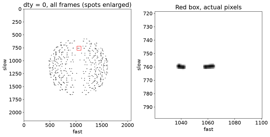
The spots stop well inside the detector because we only generated hkls up to \(d^* = 1.0\) Å\(^{-1}\) (dsmax above). At this wavelength that is \(2\theta\) = 16.4°, 587 pixels from the beam centre, while the detector reaches \(d^* \approx 1.6\) at its edges and 2.3 in its corners. A larger dsmax fills more of the detector, at the cost of more hkls to render.

As a check that the intensities land where the forward model says they should, we mark the centroid (slow, fast) of every selected peak on top of them:

def centroid_of(entry, hkl_index, branch):
    ubi, pos, hkl = ent["ubi"][entry], ent["pos"][entry], jnp.asarray(hkls)[hkl_index]
    return anri.fwd.get_centroid_box(ubi, pos, hkl, 1.0 - 2.0 * branch, *beam_and_gonio, *detector)[0]

centroids = np.asarray(jax.jit(jax.vmap(centroid_of))(e, h, b))  # (slow, fast, omega) of every selected peak

def show(ax, half, marker_size):
    # rendered intensities (actual pixels) within `half` pixels of our peak, and the centroids of the peaks there
    ax.imshow(np.log10(1 + image[s - half : s + half, f - half : f + half]), cmap="gray_r",
              extent=(f - half - 0.5, f + half - 0.5, s + half - 0.5, s - half - 0.5))
    near = (np.abs(centroids[:, 0] - s) < half) & (np.abs(centroids[:, 1] - f) < half)
    ax.scatter(centroids[near, 1], centroids[near, 0], s=marker_size, c="r", marker=".", linewidths=0)
    ax.set(title=f"{2 * half} x {2 * half} pixels: {near.sum()} peak centroids", xlabel="fast", ylabel="slow")

fig, axs = plt.subplots(1, 2, figsize=(11, 5.5), constrained_layout=True)
show(axs[0], 150, 0.5)
show(axs[1], 40, 2)
plt.show()

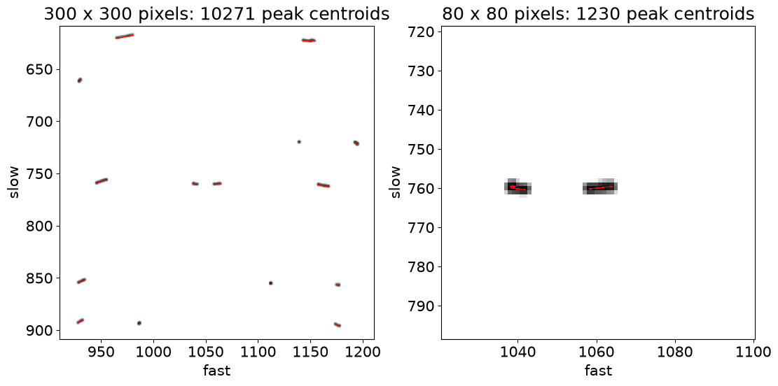
In both regions, every spot sits on the centroids of its peaks, and there are no centroids without a spot.

A whole scan

anri.io.simulate_sparse runs render_row for each row of a scan and writes ImageD11’s sparse pixel format, one group per row ("1.1", "2.1", …). Values are rounded to counts, and only counts above cut are kept. anri.io.write_pars, anri.io.write_zero_distortion, anri.io.write_dataset and anri.io.write_peaks_table then make the parameter, DataSet and peaks table files that ImageD11’s S3DXRD pipeline expects. tests/unit/io/test_imaged11.py runs that whole chain.

Here we simulate the three rows nearest the centre of the sample, into a temporary folder:

omega_grid, dty_grid = anri.io.motor_grid((0.0, 180.0), ostep, (-geom["voxel_size"], geom["voxel_size"]), geom["voxel_size"])
print("motor grid (rows, frames):", omega_grid.shape)

from ImageD11.sparseframe import SparseScan

with tempfile.TemporaryDirectory() as tmp:
    path = os.path.join(tmp, "sparse.h5")
    scan_stats = anri.io.simulate_sparse(path, entries, hkls, F2, geom, omega_grid, dty_grid, det_shape)
    print("pixels written per row:", scan_stats["n_pixels"])
    scan = SparseScan(path, "2.1")  # the middle row, read back by ImageD11
    print("ImageD11 reads", scan.shape, "with", scan.nnz.sum(), "non-zero pixels")

motor grid (rows, frames): (3, 720)
pixels written per row: [30685 30576 30511]
ImageD11 reads (720, 2162, 2068) with 30576 non-zero pixels

Settings you may need to change

• The beam and the voxels: geom_from_pars takes the beam’s profile across it (sig_beam, width_beam horizontally, sig_beam_v, width_beam_v vertically) and voxel_3d for maps of cubes. A pencil beam is narrow both ways, a line beam wide one way, a box beam (e.g. for DCT) wider than the sample both ways; k_in_lab sets its direction.

• ``window`` (default (3, 7, 7) frames × pixels × pixels): peaks broader than their window lose their tails. Check stats["captured"] from render_row, or run check_render. Peaks that are broad in \(\omega\), near \(\eta\) = 0° or 180°, need more frames.

• The intensity scale, ``min_value`` and ``cut``: rendered values are density × \(|F|^2\) × \(L\) × \(P\) × \(w_\text{beam}\) × (fraction of the peak), so their scale is set by the densities you give the map. render_row drops contributions below min_value (default \(10^{-3}\)) before merging peaks, and simulate_sparse rounds to integer counts and keeps those above cut (default 1). Choose densities that give realistic counts, or faint peaks disappear.

• ``batch``: how many peaks are rendered at once. anri.fwd.guess_batch_size picks the largest that fits in a fraction of the free memory (default 25%).

• ``anri.utils.setup(n_cpu=4)``: the number of XLA CPU devices that the work is split over.

Speed, memory and devices

• Call ``anri.utils.setup()`` first, before JAX computes anything. It sets the number of XLA CPU devices that rows are split over, stops JAX reserving most of the GPU memory at start-up, and, with jaxlib 0.11 or newer, turns off XLA:CPU fusions that miscompile the renderer.

• ``batch`` is the number of peaks rendered at once, over all devices. Each peak produces one value per window cell (3 × 7 × 7 = 147 by default), so memory grows with batch × window cells: anri.fwd.guess_batch_size measures it for your problem.

• Precision: this notebook runs in float32, JAX’s default. With float64 (jax.config.update("jax_enable_x64", True)) every number printed here agrees to within a few parts in \(10^4\), at twice the memory.

• Gradients: pixel values are differentiable with respect to the map (UBI, position, density) and the geometry. Which pixels a peak touches is not: the window is placed from rounded centroids.

print(f"Took {time.time() - start:.0f} seconds")

Took 81 seconds