Forward model with errors#
As a forward model is basically just a change-of-basis (\((h,k,l)\) space to detector space), we can propagate an error in the change-of-basis matrix (such as an error in wavelength) through the forward model to understand how our peak positions change as a function of our input parameters.
[1]:
import os
os.environ["XLA_PYTHON_CLIENT_PREALLOCATE"] = "0"

import jax
jax.config.update("jax_enable_x64", True)
import jax.numpy as jnp
from jax.scipy.spatial.transform import Rotation as jR
from matplotlib import pyplot as plt

import anri.crystal, anri.geom, anri.diffract

import time

start = time.time()
Crystallography#
Let’s do a quick and dirty generation of a single peak to forward model. We’ll choose BCC iron again:
[2]:
struc = anri.crystal.Structure.from_cif("../../../tests/data/cif/Fe.cif")
[3]:
# The central value of wavelength
wavelength_cen = 0.2
struc.make_hkls(dsmax=0.6, wavelength=wavelength_cen)
# just take the first peak:
hkl = struc.ringhkls_arr[0]
print(hkl)
[1 0 1]
We’ll generate a single grain at the origin with a known orientation:
[4]:
U = jnp.eye(3)
UB = U @ struc.B
UBI = jnp.linalg.inv(UB)
print(UBI)
origin_sample = jnp.array([0., 0., 0.])
[[2.86303550e+00 4.60411223e-16 4.60411223e-16]
 [0.00000000e+00 2.86303550e+00 1.75310363e-16]
 [0.00000000e+00 0.00000000e+00 2.86303550e+00]]
Experiment parameters#
In this simple experiment, all our parameters are constant:
[5]:
# goniometer
chi = 0.0
wedge = 0.0
dty = 0.0
y0 = 0.0
# detector
y_center = 1024.0
z_center = 1024.0
y_size = 75.0
z_size = 75.0
tilt_x = 0.0
tilt_y = 0.0
tilt_z = 0.0
distance = 300e3
o11 = 1
o12 = 0
o21 = 0
o22 = 1
detector_size = 2048  # px
[6]:
det_trans, beam_cen_shift, x_distance_shift = anri.geom.detector_transforms(
y_center,
y_size,
tilt_y,
z_center,
z_size,
tilt_z,
tilt_x,
distance,
o11,
o12,
o21,
o22
)

sc_lab, fc_lab, norm_lab = anri.geom.detector_basis_vectors_lab(det_trans, beam_cen_shift, x_distance_shift)
Let’s define a simple function in JAX to forward model a single HKL with variable wavelength:
[7]:
@jax.jit
def simulate_one_peak(ubi, hkl, origin, wavelength):
    # origin: sample frame
    q_sample = jnp.linalg.inv(ubi) @ hkl

    k_in_lab = jnp.array([1., 0., 0.])
    k_in_lab_norm = anri.diffract.scale_norm_k(k_in_lab, wavelength)
    k_in_sample_norm = anri.geom.lab_to_sample(k_in_lab_norm, 0.0, wedge, chi, dty, y0)

    omega, valid1 = anri.diffract.omega_solns(q_sample, 1.0, k_in_sample_norm)

    q_lab = anri.geom.sample_to_lab(q_sample, omega, wedge, chi, dty, y0)

    _, eta = anri.diffract.q_lab_to_tth_eta(q_lab, wavelength)
    jax.debug.print("eta (deg): {eta}", eta=eta)

    origin_lab = anri.geom.sample_to_lab(origin, omega, wedge, chi, dty, y0)

    k_out = anri.diffract.q_lab_to_k_out(q_lab, k_in_lab_norm)

    sc, fc = anri.geom.raytrace_to_det(k_out, origin_lab, sc_lab, fc_lab, norm_lab)

    return jnp.array([sc, fc, omega])
[8]:
sc, fc, omega = simulate_one_peak(UBI, hkl, origin_sample, wavelength_cen)
eta (deg): 44.92993025447665
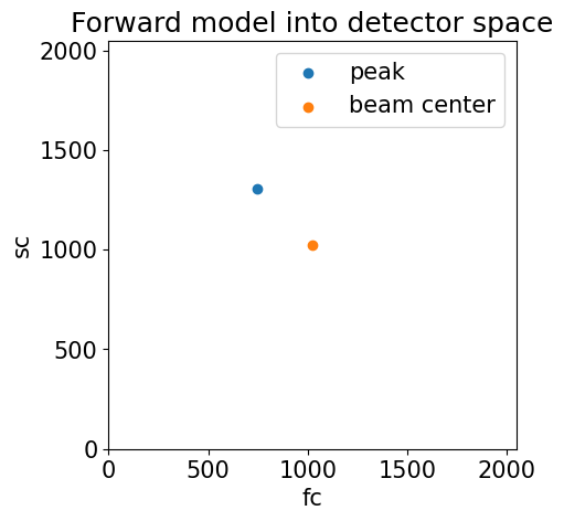
[9]:
fig ,ax = plt.subplots()
ax.scatter(fc, sc, label='peak')
ax.scatter(y_center, z_center,label='beam center')
ax.set(ylim=(0, detector_size), xlim=(0, detector_size), aspect=1, title='Forward model into detector space', xlabel='fc', ylabel='sc')
ax.legend()
plt.show()
Understanding error propagation#
\(\mathbf {f} :\mathbb {R} ^{n}\to \mathbb {R} ^{m}\)
This notation means that the function \(\mathbf{f}\) takes a length-\(n\) vector of real numbers and returns another length-\(m\) vector of real numbers.
We can represent the input as some length-\(n\) vector:
\(\mathbf {x} =(x_{1},\ldots ,x_{n})\in \mathbb {R} ^{n}\)
and the output as a length-\(m\) vector:
\(\mathbf {f} (\mathbf {x} )=(f_{1}(\mathbf {x} ),\ldots ,f_{m}(\mathbf {x} ))\in \mathbb {R} ^{m}\)
We can then define the Jacobian matrix \(\mathbf {J_{f}}\):
\(\mathbf {J_{f}} ={\begin{bmatrix}{\dfrac {\partial \mathbf {f} }{\partial x_{1}}}&\cdots &{\dfrac {\partial \mathbf {f} }{\partial x_{n}}}\end{bmatrix}}={\begin{bmatrix}\nabla ^{\mathsf {T}}f_{1}\\\vdots \\\nabla ^{\mathsf {T}}f_{m}\end{bmatrix}}={\begin{bmatrix}{\dfrac {\partial f_{1}}{\partial x_{1}}}&\cdots &{\dfrac {\partial f_{1}}{\partial x_{n}}}\\\vdots &\ddots &\vdots \\{\dfrac {\partial f_{m}}{\partial x_{1}}}&\cdots &{\dfrac {\partial f_{m}}{\partial x_{n}}}\end{bmatrix}}\)
The above means that \(\mathbf {J_{f}}\) encodes the partial derivatives of each value of the output vector \(\mathbf {f} (\mathbf {x} )\) with respect to each value of the input vector \(\mathbf {x}\).
As a very basic example:
\(\mathbf {f}(x, y) = \mathbf (x^2, y^2)\)
The Jacobian would then be:
\(\mathbf {J_{f}} = {\begin{bmatrix}{\dfrac {\partial f_{1}}{\partial x_{1}}} &{\dfrac {\partial f_{1}}{\partial x_{2}}}\\ {\dfrac {\partial f_{2}}{\partial x_{1}}} &{\dfrac {\partial f_{2}}{\partial x_{2}}}\end{bmatrix}}\)
For \((x_1, x_2) = (x, y)\) and \((f_1, f_2) = (x^2, y^2)\) we then get:
\(\mathbf {J_{f}} = {\begin{bmatrix}{\dfrac {\partial x^2}{\partial x}} & {\dfrac {\partial x^2}{\partial y}}\\ {\dfrac {\partial y^2}{\partial x}} &{\dfrac {\partial y^2}{\partial y}}\end{bmatrix}} = \begin{bmatrix}2x & 0 \\ 0 & 2y\end{bmatrix}\)
Let’s now see how to implement this in Jax:
[10]:
@jax.jit
def f(vec_in):
    vec_out = jnp.power(vec_in, 2)
    return vec_out

vec_in = jnp.array([2.0, 3.0])
vec_out = f(vec_in)
print(vec_out)
[4. 9.]
We can manually define the Jacobian:
[11]:
@jax.jit
def jac_func_manual(vec_in):
    vec_out = jnp.array([
        [2*vec_in[0], 0],
        [0, 2*vec_in[1]]
    ])
    return vec_out
Now we define a function in JAX that can give us the Jacobian:
[12]:
jac_func = jax.jacfwd(f)

J = jac_func(vec_in)

print(J)
[[4. 0.]
 [0. 6.]]
And we can check that our manual Jacobian function agrees:
[13]:
J_manual = jac_func_manual(vec_in)

print(J_manual)

assert jnp.allclose(J, J_manual)
[[4. 0.]
 [0. 6.]]
Now let’s assume we have some uncertainty in our inputs.
We can generate a variance-covariance matrix on our inputs:
\(\mathbf{\Sigma}^{\text{in}} = \begin{pmatrix} \sigma_x^2 & \sigma_{xy} \\ \sigma_{yx} & \sigma_y^2 \end{pmatrix}\)
We can propagate our errors in the input vector to the errors in the output vector:
\(\mathbf{\Sigma}^{\text{out}} = \mathbf {J_{f}} \mathbf{\Sigma}^{\text{in}} \mathbf {J_{f}}^T\)
We can convince ourselves of this via JAX:
[14]:
sig_x = 1.0
sig_y = 2.0
# assume linearly independent:
cov_in = jnp.array([[sig_x**2, 0], [0, sig_y**2]])

cov_out = J @ cov_in @ J.T

print(cov_out)
[[ 16.   0.]
 [  0. 144.]]
For a simple function \(f=A^b\), the variance in \(f\), \(\sigma_f^2\) goes as:
\(\sigma_f^2 = \left(\frac{f b \sigma_A}{A}\right)^2\)
We can check that our output covariance matrix matches:
[15]:
assert jnp.allclose(cov_out[0,0], (vec_out[0] * 2 * sig_x / vec_in[0])**2)

assert jnp.allclose(cov_out[1,1], (vec_out[1] * 2 * sig_y / vec_in[1])**2)
We have now shown that we can use JAX to propagate errors in parameters through arbitrary functions.
Forward propagating errors#
To keep things simple-ish, let’s assume there are two sources of error:
origin_sample- we can move the grain around in space. This shouldn’t change the Bragg angle, but it will change the peak position on the detector linearly.wavelength- this will change all of(sc, fc omega)
For now, we’ll say the wavelength is perfect, just to inspect the effect of the error in grain position.
First, we use JAX to get a function that yields the Jacobian of our forward simulation:
[16]:
jac_func = jax.jacfwd(simulate_one_peak, argnums=(2,3))
Then we call the function on the peak position to get the actual Jacobian:
[17]:
J_origin, J_wav = jac_func(UBI, hkl, origin_sample, wavelength_cen)
eta (deg): 44.92993025447665
As we are investigating two parameters, we get two Jacobians. We can combine them together into a single 4x4 matrix:
[18]:
J_wav = J_wav.reshape(3,1)
J_total = jnp.block([J_origin, J_wav])
Now we write a quick function that gives us the covariance matrices given some observed standard deviations in our experimental parameters:
[19]:
from jax.scipy.linalg import block_diag

def get_cov(sig_wav, sig_origin):
    cov_beam = jnp.array([[sig_wav**2]])
    cov_origin = jnp.eye(3) * (sig_origin**2)

    # combine together into one covariance matrix:
    cov_total = block_diag(cov_origin, cov_beam)
    return cov_total
Now with the Jacobian and covariance matrices, we can combine them together to project the covariance matrix into detector space:
[20]:
# Standard deviations for beam
sig_wav = 0.0  # same units as wavelength_cen
# Standard deviations for grain position (assume isotropic in all three directions):
sig_origin = 75.0

cov_total = get_cov(sig_wav, sig_origin)
[21]:
cov_det = J_total @ cov_total @ J_total.T
print('Covariance matrix in detector space:')
print(cov_det)
Covariance matrix in detector space:
[[ 1.00492783 -0.00491579  0.        ]
 [-0.00491579  1.00490378  0.        ]
 [ 0.          0.          0.        ]]
We can now investigate the result. As we specified the standard deviation of the origin to be equal to the pixel size, we can expect the standard deviations on (sc, fc) to be approximately 1 pixel, and for the Bragg angle to be unaffected:
[22]:
sig_sc, sig_fc, sig_omega = jnp.sqrt(jnp.diag(cov_det))
print('(sig_sc, sig_fc, sig_omega):')
print(sig_sc, sig_fc, sig_omega)
(sig_sc, sig_fc, sig_omega):
1.0024608857047221 1.0024488916182213 0.0
We see that the errors in detector space are close to 1, but not exactly. This is probably due to the assumption in linearity imposed by the Jacobian-covariance matrix product we used earlier.
Now let’s introduce variable wavelength:
[23]:
# Standard deviations for beam
sig_wav = 1e-5  # more realistic for ID11
# Standard deviations for grain position (assume isotropic in all three directions):
sig_origin = 0.0

cov_total = get_cov(sig_wav, sig_origin)

cov_det = J_total @ cov_total @ J_total.T
print('Covariance matrix in detector space:')
print(cov_det)

sig_sc, sig_fc, sig_omega = jnp.sqrt(jnp.diag(cov_det))
print('(sig_sc, sig_fc, sig_omega):')
print(sig_sc, sig_fc, sig_omega)
Covariance matrix in detector space:
[[ 2.00998452e-04 -1.99533736e-04 -2.84416309e-06]
 [-1.99533736e-04  1.98079694e-04  2.82343710e-06]
 [-2.84416309e-06  2.82343710e-06  4.02454028e-08]]
(sig_sc, sig_fc, sig_omega):
0.014177392282315614 0.01407407879855225 0.00020061256895798654
sc and fc to be equal as we change the wavelength. Combining both together with more realistic numbers:[24]:
# Standard deviations for beam
sig_wav = 1e-5  # more realistic for ID11
# Standard deviations for grain position (assume isotropic in all three directions):
sig_origin = 10.0

cov_total = get_cov(sig_wav, sig_origin)

cov_det = J_total @ cov_total @ J_total.T
print('Covariance matrix in detector space:')
print(cov_det)

sig_sc, sig_fc, sig_omega = jnp.sqrt(jnp.diag(cov_det))
print('(sig_sc, sig_fc, sig_omega):')
print(sig_sc, sig_fc, sig_omega)
Covariance matrix in detector space:
[[ 1.80663820e-02 -2.86925543e-04 -2.84416309e-06]
 [-2.86925543e-04  1.80630358e-02  2.82343710e-06]
 [-2.84416309e-06  2.82343710e-06  4.02454028e-08]]
(sig_sc, sig_fc, sig_omega):
0.1344112422737702 0.13439879385012135 0.00020061256895798654
So we can see that a variance in the wavelength of around \(10^{-5}\) and a variance in grain position of around 10 µm changes the pixel position by around 0.13 pixels with this current detector setup.