Simple forward model#
Now we have some crystallographic functions and we can handle the detector geometry, we can perform a basic forward model of a single crystal to reassure ourselves that this wasn’t all for nothing!
[1]:
import os
os.environ["XLA_PYTHON_CLIENT_PREALLOCATE"] = "0"

import jax
jax.config.update("jax_enable_x64", True)
import jax.numpy as jnp
from jax.scipy.spatial.transform import Rotation as jR
from matplotlib import pyplot as plt

import anri.crystal, anri.geom, anri.diffract

import time

start = time.time()
Anri, all fundamental functions and transforms are written for single vectors.[2]:
# easy example: many hkls, single B matrix, so we vmap over hkls only, giving us [0, None]
omega_solns_vec = jax.vmap(anri.diffract.omega_solns, in_axes=[0, None, None])
sample_to_lab_vec = jax.vmap(anri.geom.sample_to_lab, in_axes=[0, 0, None, None, None, None])
q_lab_to_k_out_vec = jax.vmap(anri.diffract.q_lab_to_k_out, in_axes=[0, None])
raytrace_to_det_vec = jax.vmap(anri.geom.raytrace_to_det, in_axes=[0, None, None, None, None])
q_lab_to_tth_eta_vec = jax.vmap(anri.diffract.q_lab_to_tth_eta, in_axes=[0, None])
Crystallography#
Let’s take a simple Fe CIF file
[3]:
struc = anri.crystal.Structure.from_cif("../../../tests/data/cif/Fe.cif")
We generate some hkls:
[4]:
dsmax = 2.0
wavelength = 0.3
struc.make_hkls(dsmax=dsmax, wavelength=wavelength)
[5]:
struc.rings_dict[0]
[5]:
| h | k | l | tth | ds | intensity | ring_id |
|---|---|---|---|---|---|---|
| i64 | i64 | i64 | f64 | f64 | f64 | u32 |
| 0 | -1 | 1 | 8.498266 | 0.493956 | 1363.448082 | 0 |
| 1 | 1 | 0 | 8.498266 | 0.493956 | 1363.448082 | 0 |
| -1 | 0 | 1 | 8.498266 | 0.493956 | 1363.448082 | 0 |
| -1 | 0 | -1 | 8.498266 | 0.493956 | 1363.448082 | 0 |
| -1 | -1 | 0 | 8.498266 | 0.493956 | 1363.448082 | 0 |
| … | … | … | … | … | … | … |
| 1 | -1 | 0 | 8.498266 | 0.493956 | 1363.448082 | 0 |
| 0 | -1 | -1 | 8.498266 | 0.493956 | 1363.448082 | 0 |
| 0 | 1 | -1 | 8.498266 | 0.493956 | 1363.448082 | 0 |
| 0 | 1 | 1 | 8.498266 | 0.493956 | 1363.448082 | 0 |
| -1 | 1 | 0 | 8.498266 | 0.493956 | 1363.448082 | 0 |
Let’s generate a random orientation.
[6]:
key = jax.random.key(time.time_ns())
random_euler = jax.random.uniform(key, shape=(3,), minval=-90.0, maxval=90.0)
U = jR.from_euler('XYZ', random_euler, degrees=True).as_matrix()
U
[6]:
Array([[ 0.69054177,  0.67030248,  0.2717474 ],
       [-0.29615992,  0.60480449, -0.73925694],
       [-0.65987981,  0.43000711,  0.61615949]], dtype=float64)
Now we can generate some scattering vectors in the sample frame:
[7]:
UB = U @ struc.B
q_sample = (UB @ struc.ringhkls_arr.T).T
q_sample.shape
[7]:
(380, 3)
Ewald condition#
Now we can determine the omega angles required to diffract:
[8]:
chi = 0.0
wedge = 0.0
dty = 0.0
y0 = 0.0

# define incoming wavevector in the lab frame
k_in_lab = jnp.array([1., 0, 0])
k_in_lab_norm = anri.diffract.scale_norm_k(k_in_lab, wavelength)

# map it into the sample frame
k_in_sample_norm = anri.geom.lab_to_sample(k_in_lab_norm, 0.0, wedge, chi, dty, y0)
# etasign +1:
omega1, valid1 = omega_solns_vec(q_sample, 1.0, k_in_sample_norm)
# etasign -1:
omega2, valid2 = omega_solns_vec(q_sample, -1.0, k_in_sample_norm)
omega = jnp.concatenate([omega1, omega2])
valid = jnp.concatenate([valid1, valid2])
q_sample = jnp.concatenate([q_sample, q_sample])
omega_valid = omega[valid]
q_sample_valid = q_sample[valid]
Into the lab frame#
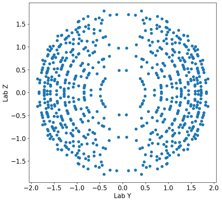
With the omega angles determined, we can rotate q_sample into the lab frame:
[9]:
q_lab = sample_to_lab_vec(q_sample_valid, omega_valid, wedge, chi, dty, y0)
[10]:
fig, ax = plt.subplots(figsize=(8,8))
ax.scatter(q_lab[:, 1], q_lab[:, 2])
ax.set_aspect(1)
ax.set(xlabel='Lab Y', ylabel='Lab Z')
plt.show()
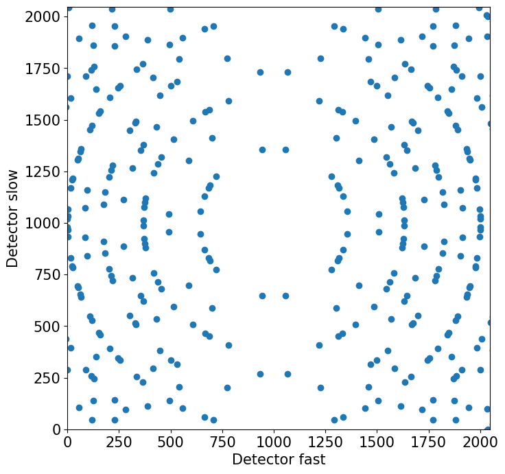
Into the detector#
Now we can forward-project them into the detector!
Let’s set up the detector transforms:
[11]:
y_center = 1000.0
z_center = 1000.0
y_size = 75.0
z_size = 75.0
tilt_x = 0.0
tilt_y = 0.0
tilt_z = 0.0
distance = 180e3
o11 = 1
o12 = 0
o21 = 0
o22 = 1
det_trans, beam_cen_shift, x_distance_shift = anri.geom.detector_transforms(
    y_center,
    y_size,
    tilt_y,
    z_center,
    z_size,
    tilt_z,
    tilt_x,
    distance,
    o11,
    o12,
    o21,
    o22
)
We get the detector basis vectors in the lab frame:
[12]:
sc_lab, fc_lab, norm_lab = anri.geom.detector_basis_vectors_lab(det_trans, beam_cen_shift, x_distance_shift)
Now we can map into detector space:
[13]:
origin_lab = jnp.array([0., 0, 0])

# get outgoing scattering vector
k_out = q_lab_to_k_out_vec(q_lab, k_in_lab_norm)
# ray-trace it into the detector
sc, fc = raytrace_to_det_vec(k_out, origin_lab, sc_lab, fc_lab, norm_lab)
Results#
[14]:
fig, ax = plt.subplots(figsize=(8,8))
ax.scatter(fc, sc)
ax.set_aspect(1)
ax.set(xlabel='Detector fast', ylabel='Detector slow')
# set some sensible detector limits
ax.set_xlim(0, 2048)
ax.set_ylim(0, 2048)
plt.show()
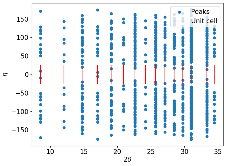
[15]:
tth, eta = q_lab_to_tth_eta_vec(q_lab, wavelength)
[16]:
fig, ax = plt.subplots(figsize=(8,6))
ax.scatter(tth, eta, label='Peaks')
ax.vlines(struc.ringtth, -25, 25, color='red', label='Unit cell')
ax.set(xlabel=r'$2\theta$', ylabel=r'$\eta$')
ax.legend(loc='upper right')
plt.show()
Index the forward-simulated peaks with ImageD11#
[17]:
import ImageD11.columnfile, ImageD11.parameters, ImageD11.unitcell, ImageD11.indexing, ImageD11.grain

# make an ImageD11 unitcell from our structure
uc = ImageD11.unitcell.unitcell(struc.lattice_parameters, struc.sgno)

# prepare a minimal columnfile - just add detector positions and omega angles
cf_obs = ImageD11.columnfile.columnfile(new=True)
cf_obs.nrows = fc.shape[0]
cf_obs.addcolumn(fc, 'fc')
cf_obs.addcolumn(sc, 'sc')
cf_obs.addcolumn(omega_valid, 'omega')

# prepare parameters object to hold our experiment state
pars = ImageD11.parameters.parameters()
# detector
pars.set('distance', distance)
pars.set('tilt_x', tilt_x)
pars.set('tilt_y', tilt_y)
pars.set('tilt_z', tilt_z)
pars.set('y_size', y_size)
pars.set('z_size', z_size)
pars.set('y_center', y_center)
pars.set('z_center', z_center)
pars.set('o11', o11)
pars.set('o12', o12)
pars.set('o21', o21)
pars.set('o22', o22)
# beam
pars.set('wavelength', wavelength)
# diffractometer
pars.set('chi', chi)
pars.set('wedge', wedge)
pars.set('t_x', 0)
pars.set('t_y', 0)
pars.set('t_z', 0)
pars.set('omegasign', 1)
cf_obs.parameters = pars
print(pars.get_parameters())
{'distance': 180000.0, 'tilt_x': 0.0, 'tilt_y': 0.0, 'tilt_z': 0.0, 'y_size': 75.0, 'z_size': 75.0, 'y_center': 1000.0, 'z_center': 1000.0, 'o11': 1, 'o12': 0, 'o21': 0, 'o22': 1, 'wavelength': 0.3, 'chi': 0.0, 'wedge': 0.0, 't_x': 0, 't_y': 0, 't_z': 0, 'omegasign': 1}
Now we compute the peak geometry with ImageD11:
[18]:
print(cf_obs.titles)
cf_obs.updateGeometry()
print(cf_obs.titles)
['fc', 'sc', 'omega']
['fc', 'sc', 'omega', 'xl', 'yl', 'zl', 'tth', 'eta', 'ds', 'gx', 'gy', 'gz']
Sanity check - we should compute the same g-vectors in the sample frame (q_sample):
[19]:
jnp.abs(jnp.stack([cf_obs.gx, cf_obs.gy, cf_obs.gz], axis=1) - q_sample_valid).max()
[19]:
Array(1.55431223e-15, dtype=float64)
Now let’s set up our indexer and run it:
[20]:
ImageD11.indexing.loglevel = 3
idx = ImageD11.indexing.indexer_from_colfile_and_ucell(cf_obs, uc)
idx.ds_tol = 0.005
idx.assigntorings()
idx.hkl_tol = 0.01
idx.score_all_pairs()
[21]:
id11_ubi = idx.ubis[0]
id11_grain = ImageD11.grain.grain(id11_ubi)
# B matrices should be very similar:
print(jnp.abs(id11_grain.B - struc.B).max())
# the U matrices that we get back should be the same under symmetry:
dU = id11_grain.U.T @ U
print(dU)
2.3266697698128234e-16
[[ 2.20935818e-16 -1.00000000e+00 -1.72839698e-16]
 [-1.00000000e+00 -4.22964125e-16 -5.12612731e-16]
 [ 5.86569913e-16  1.80253913e-16 -1.00000000e+00]]
An even simpler check is whether our UBI from Anri indexes the g-vectors from ImageD11:
[22]:
from ImageD11.cImageD11 import score
gve_id11 = jnp.stack([cf_obs.gx, cf_obs.gy, cf_obs.gz], axis=1)
score_result = score(ubi=jnp.linalg.inv(U @ struc.B), gv=gve_id11, tol=0.01)
print(f'Score result: {score_result}, Peaks in dataset: {cf_obs.nrows}')
Score result: 748, Peaks in dataset: 748
created an array from object
created an array from object
[23]:
end = time.time()
print(f'Took {(end - start):.1f} seconds')
Took 5.1 seconds