Goniometer geometry#
We can investigate how to convert to and from the lab and translated/rotated reference frames here.
[1]:
import os
os.environ["XLA_PYTHON_CLIENT_PREALLOCATE"] = "0"

from matplotlib import pyplot as plt

import jax
import jax.numpy as jnp

import anri.geom
Let’s get some useful basis vectors:
[2]:
e1, e2, e3 = jnp.eye(3)
e1, e2, e3
[2]:
(Array([1., 0., 0.], dtype=float32),
 Array([0., 1., 0.], dtype=float32),
 Array([0., 0., 1.], dtype=float32))
[3]:
vecs = jnp.stack((e1, e2, e3))
vecs
[3]:
Array([[1., 0., 0.],
       [0., 1., 0.],
       [0., 0., 1.]], dtype=float32)
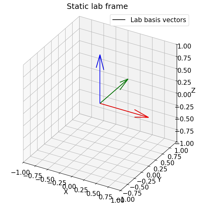
And we’ll whip up a quick function to plot some 3D vectors in the lab frame.
[4]:
def plot_vectors_3d(vec, origin=None, legend=''):
    if origin is None:
        origin = jnp.zeros_like(vec)
    ax = plt.figure(figsize=(8,8)).add_subplot(projection='3d',)
    ax.set_proj_type('ortho')
    ax.quiver([0, 0, 0], [0, 0, 0], [0, 0, 0], [1, 0, 0], [0, 1, 0], [0, 0, 1], color='k', label='Lab basis vectors')
    uv = vec - origin
    ax.quiver(origin[:, 0], origin[:, 1], origin[:, 2],
    uv[:, 0], uv[:, 1], uv[:, 2], color=list('rgbcmyk'[:len(vec)]), label=legend)
    ax.set_xlim(-1, 1)
    ax.set_ylim(-1, 1)
    ax.set_zlim(-1, 1)
    ax.set_aspect('equal')
    ax.set_box_aspect((1,1,1))
    ax.set(xlabel='X', ylabel='Y', zlabel='Z', title='Static lab frame')

    ax.legend()
    plt.show()
[5]:
plot_vectors_3d(vecs, None, '')
Now let’s investigate how it looks when we rotate the goniometer. We can take the basis vectors for the sample (rotating) frame, and map them into the lab frame:
\(R_z(\phi) \cdot v_{\text{sample}} = v_{\text{lab}}\)
To apply this transform to many vectors at once, we need to vmap the core function over an extra axis.
[6]:
# broadcast over (npks, 3)
sample_to_lab_vec = jax.vmap(anri.geom.sample_to_lab, in_axes=(0, None, None, None, None, None))
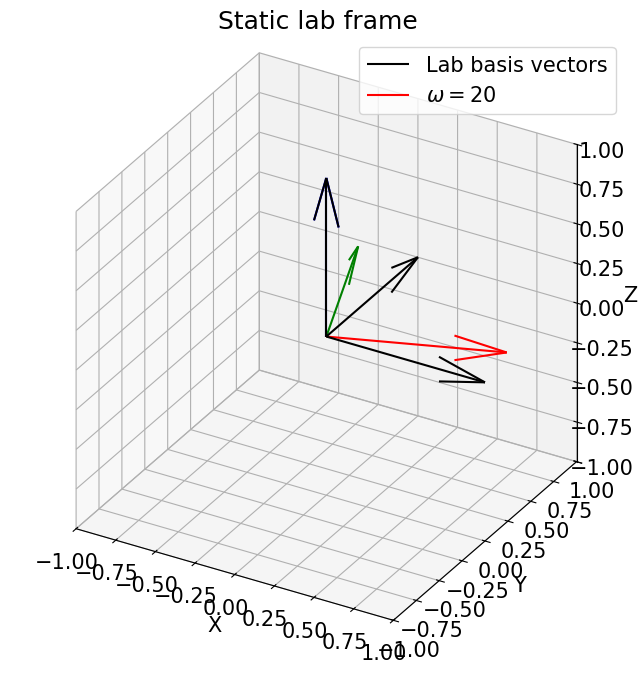
We can try a small omega rotation (10 degrees) to see how it’ll look:
[7]:
omega = 20
origin_lab = sample_to_lab_vec(jnp.zeros_like(vecs), omega, 0, 0, 0, 0)
vec_lab = sample_to_lab_vec(vecs, omega, 0, 0, 0, 0)
plot_vectors_3d(vec_lab,origin_lab, fr'$\omega={omega}$')
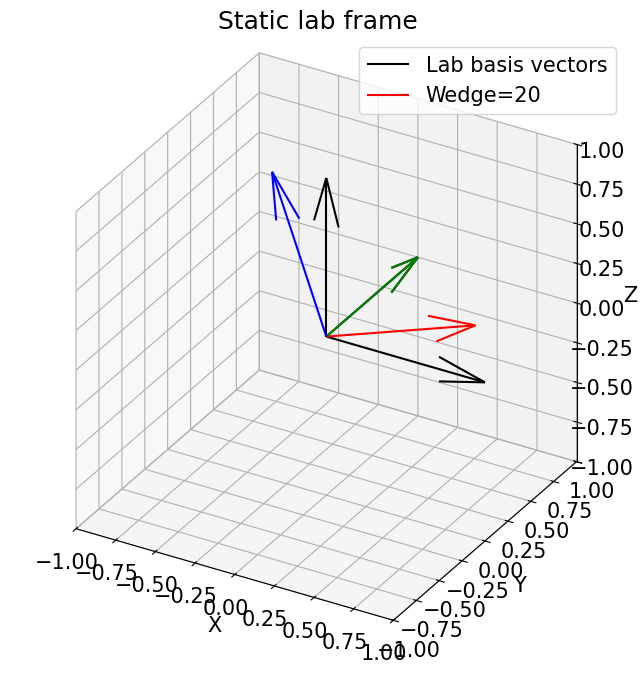
How about the wedge and omega angles?
[8]:
omega = 0
wedge = 20
origin_lab = sample_to_lab_vec(jnp.zeros_like(vecs), omega, wedge, 0, 0, 0)
vec_lab = sample_to_lab_vec(vecs, omega, wedge, 0, 0, 0)
plot_vectors_3d(vec_lab,origin_lab, f'Wedge={wedge}')
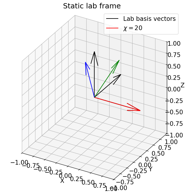
[9]:
omega = 0
wedge = 0
chi = 20
origin_lab = sample_to_lab_vec(jnp.zeros_like(vecs), omega, wedge, chi, 0, 0)
vec_lab = sample_to_lab_vec(vecs, omega, wedge, chi, 0, 0)
plot_vectors_3d(vec_lab,origin_lab, fr'$\chi={chi}$')
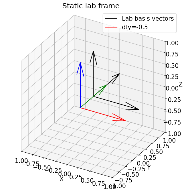
We can also investigate the effect of changing dty, which translates the whole diffractometer:
[10]:
omega = 0
wedge = 0
chi = 0
dty = -0.5
origin_lab = sample_to_lab_vec(jnp.zeros_like(vecs), omega, wedge, chi, dty, 0)
vec_lab = sample_to_lab_vec(vecs, omega, wedge, chi, dty, 0)
plot_vectors_3d(vec_lab,origin_lab, f'dty={dty}')
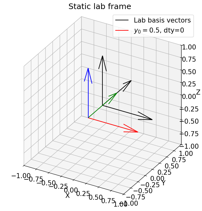
As \(y_0\) is the motor value of dty when the rotation axis hits the beam, we can investigate what happens when it’s non-zero:
[11]:
omega = 0
wedge = 0
chi = 0
dty = 0
y0 = 0.5
origin_lab = sample_to_lab_vec(jnp.zeros_like(vecs), omega, wedge, chi, dty, y0)
vec_lab = sample_to_lab_vec(vecs, omega, wedge, chi, dty, y0)
plot_vectors_3d(vec_lab,origin_lab, f'$y_0={y0}$, dty={dty}')
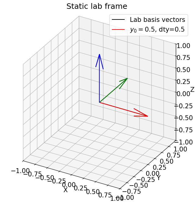
[12]:
omega = 0
wedge = 0
chi = 0
dty = 0.5
y0 = 0.5
origin_lab = sample_to_lab_vec(jnp.zeros_like(vecs), omega, wedge, chi, dty, y0)
vec_lab = sample_to_lab_vec(vecs, omega, wedge, chi, dty, y0)
plot_vectors_3d(vec_lab,origin_lab, f'$y_0={y0}$, dty={dty}')
[ ]: